Diagnostic plots

ComBat-refQL stores detailed diagnostics during fitting. ggplot2::autoplot() provides a compact visual interface to the main diagnostics without requiring users to manually extract the underlying tables.

GFRN benchmark

This vignette uses a compact subset of the real Growth Factor Receptor Network (GFRN) RNA-seq dataset used in the ComBat-seq and ComBat-ref real-data benchmarks. Human mammary epithelial cells were transfected with HER2, EGFR, KRAS, or GFP control constructs across three experimental batches. GFP controls are represented across batches, making the dataset a useful real-world example of technical batch structure alongside known biological perturbations. The original data are available from GEO under GSE83083 and GSE59765.

The original GFRN study is Activity of distinct growth factor receptor network components in breast tumors uncovers two biologically relevant subtypes. Related methods are described in the ComBat-seq paper and the ComBat-ref paper. The bundled object was prepared from the commit-pinned ComBat-ref repository using its real_data_application/signature_data.rds source file.

To keep package builds lightweight, the package bundles a deterministic subset of 1,000 well-supported genes while retaining all 47 selected samples, their original count values, batch labels, and biological labels. The preparation script uses genes observed with a positive count in every selected sample, then orders eligible genes by decreasing mean count with gene IDs as deterministic tie-breakers. It does not select genes using correction results, differential expression, or visual appearance.

gfrn_file <- system.file(
  "extdata",
  "gfrn-vignette.rds",
  package = "combatrefql"
)

gfrn <- readRDS(gfrn_file)

fit <- combat_ref_ql(
  gfrn$counts,
  batch = gfrn$batch,
  group = gfrn$group,
  verbose = FALSE
)

The bundled subset retains the biological labels gfp, her2, egfr, and kraswt and the original batch labels 1, 2, and 3. It is provided solely as a compact reproducible documentation example; it is not the complete GFRN dataset and does not imply that ComBat-refQL generated the original data.

Diagnostic overview

ggplot2::autoplot(fit)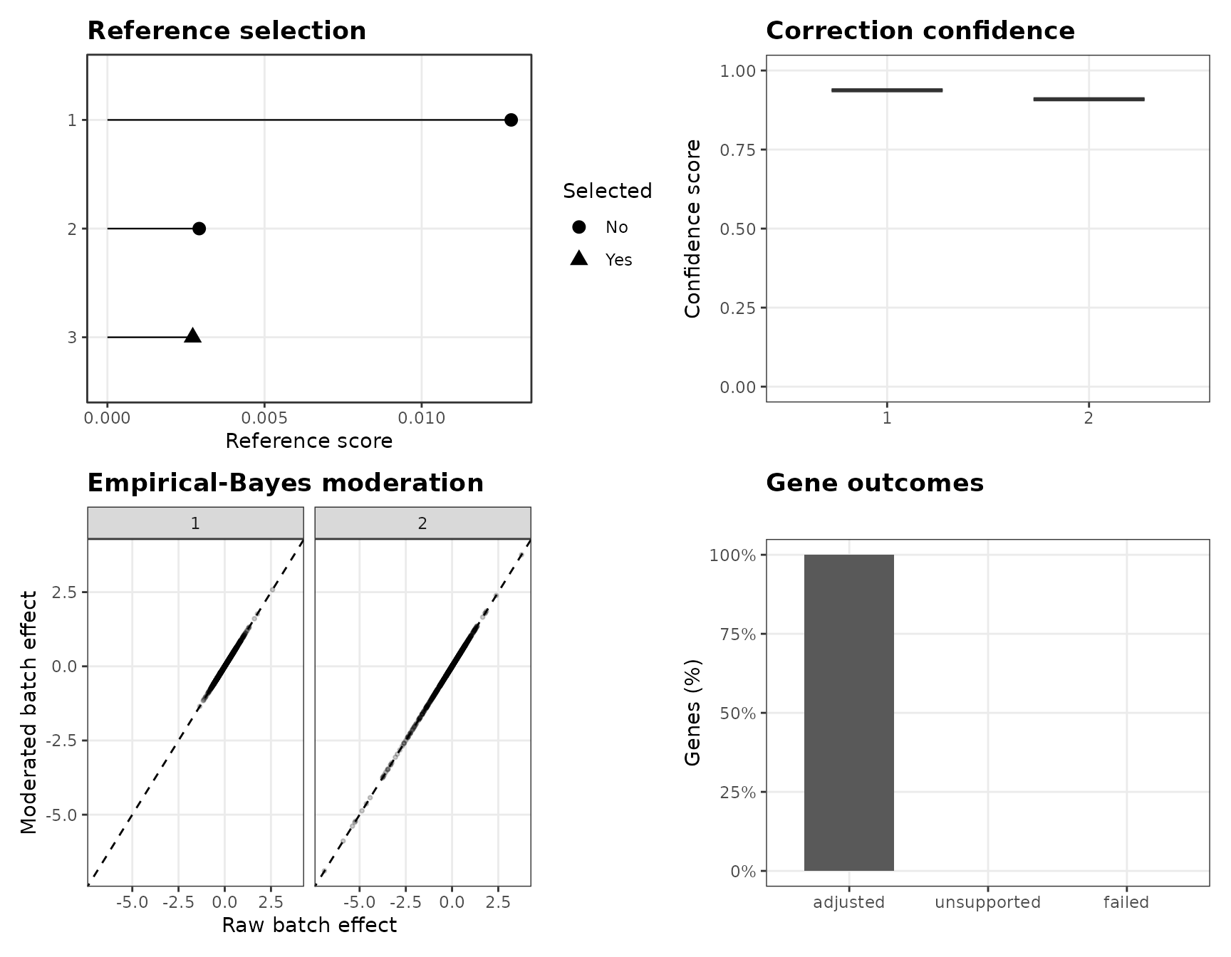

The default overview is the first visual QC step after fitting. It combines reference selection, correction confidence, empirical-Bayes moderation, and gene outcomes. These are model and correction diagnostics; they do not by themselves establish complete batch removal or preservation of every biological signal.

Understanding the overview

Panel	Diagnostic	Interpretation
Reference selection	Batch reference scores	Why a particular batch was selected
Correction confidence	Confidence-score distributions	Statistical support for source-to-reference corrections
Empirical-Bayes moderation	Raw versus posterior batch effects	Degree of moderation
Gene outcomes	Adjusted, unsupported, and failed genes	Overall correction outcome

For the score definition and its limitations, see Input sanity and correction confidence. The reference criterion and moderation model are described in Method.

Individual diagnostics

Reference selection

ggplot2::autoplot(fit, type = "reference")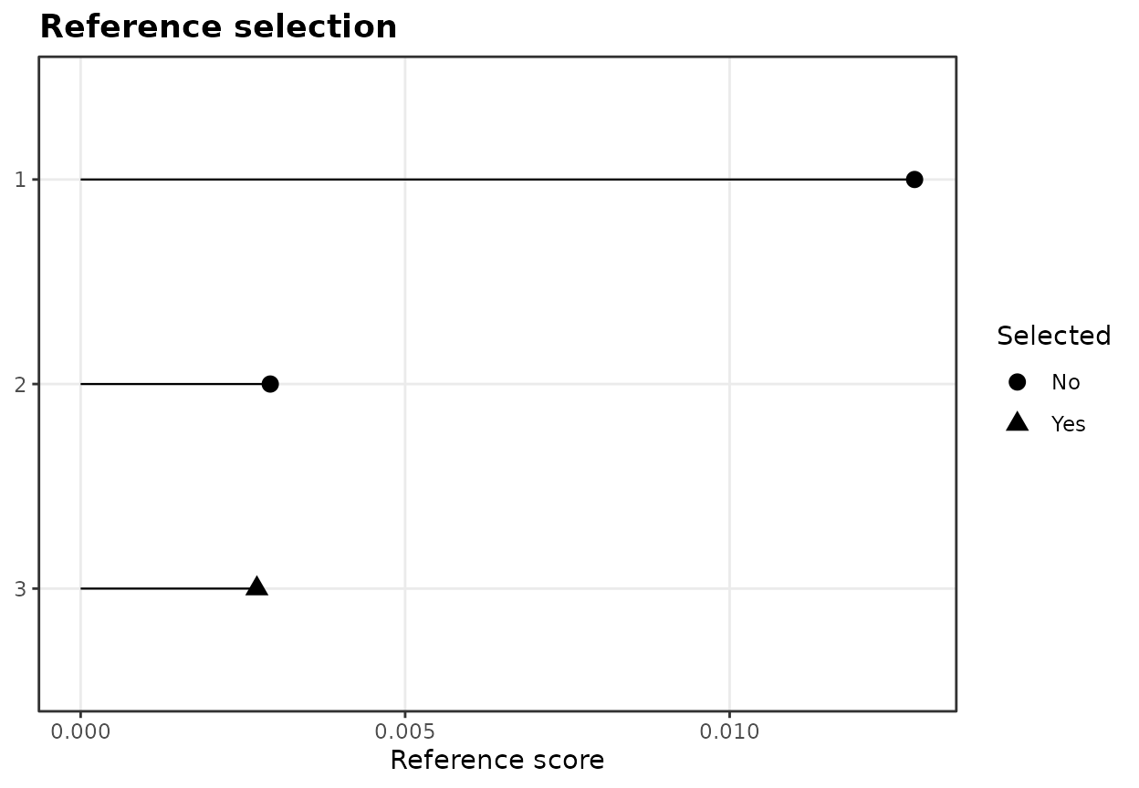

Each point is a batch and the x-axis is its reference-selection score. The selected batch is marked directly in the plot. Automatic selection uses the package’s biologically adjusted within-batch criterion; the score is intended to explain the algorithm’s choice, not to define a universally best batch outside that criterion.

Correction confidence

ggplot2::autoplot(fit, type = "confidence")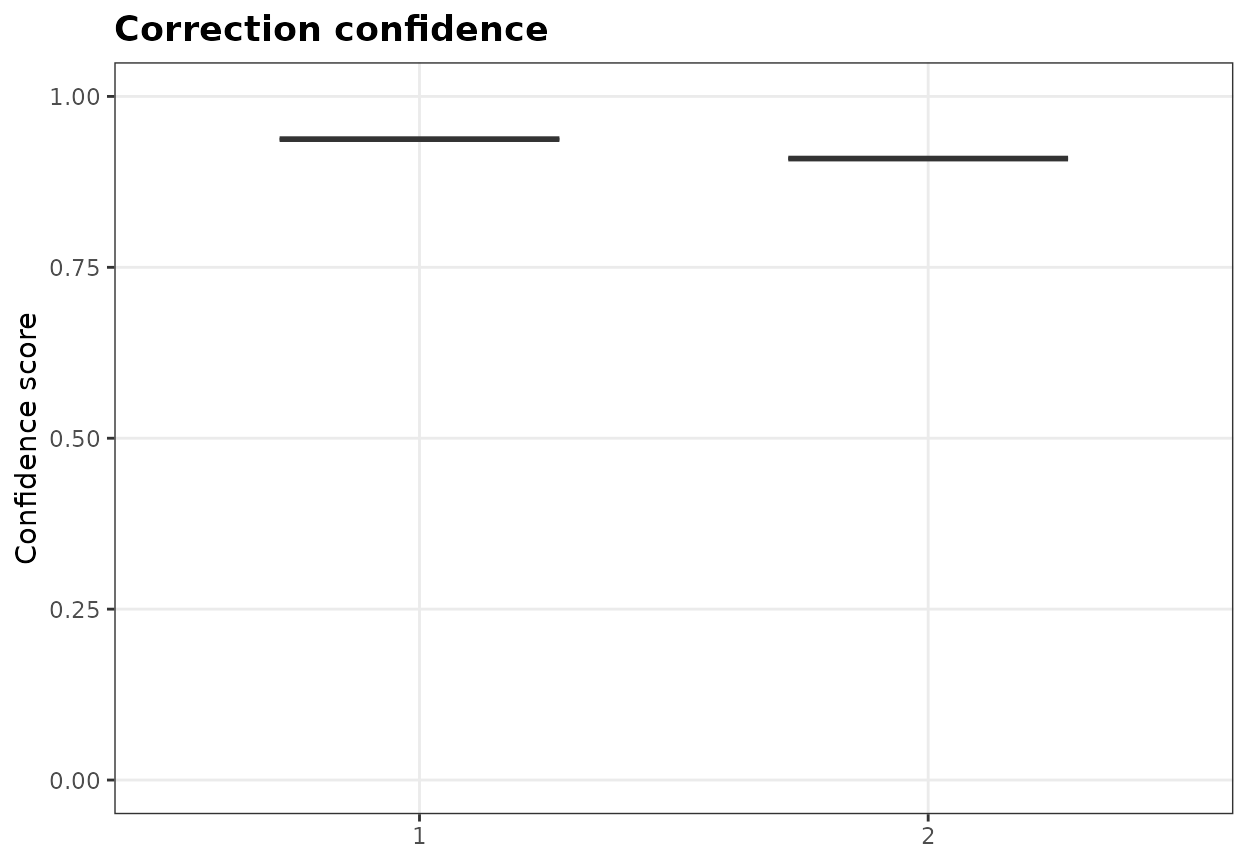

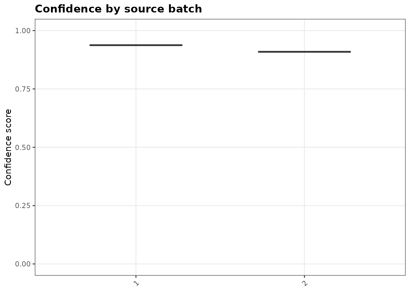
Scores summarize each gene-by-source-batch correction and range from 0 to 1. The boxplots show their distribution for each source batch. Lower scores can reflect limited replication, weak residual information, dispersion fallback, or mapping problems. The confidence score is a reliability/support diagnostic, not a posterior probability or p-value. See Input sanity and correction confidence for the exact definition.

Empirical-Bayes moderation

ggplot2::autoplot(fit, type = "shrinkage")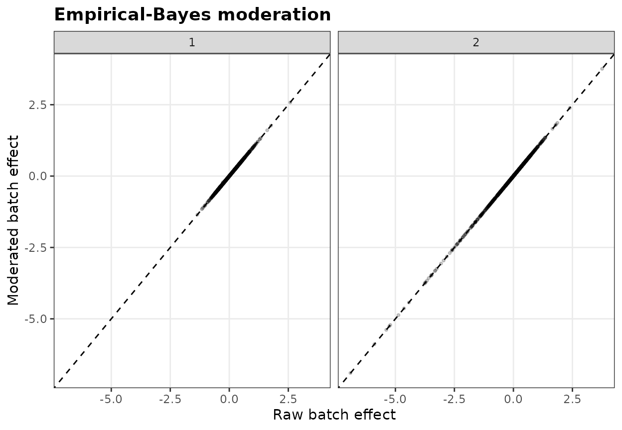

The dashed line is the identity line. Points near it changed little after moderation; deviations show how the raw batch-effect estimate changed after empirical-Bayes moderation. Each facet is a source batch, making it easier to see how moderation stabilizes noisy estimated effects.

Gene outcomes

ggplot2::autoplot(fit, type = "outcomes")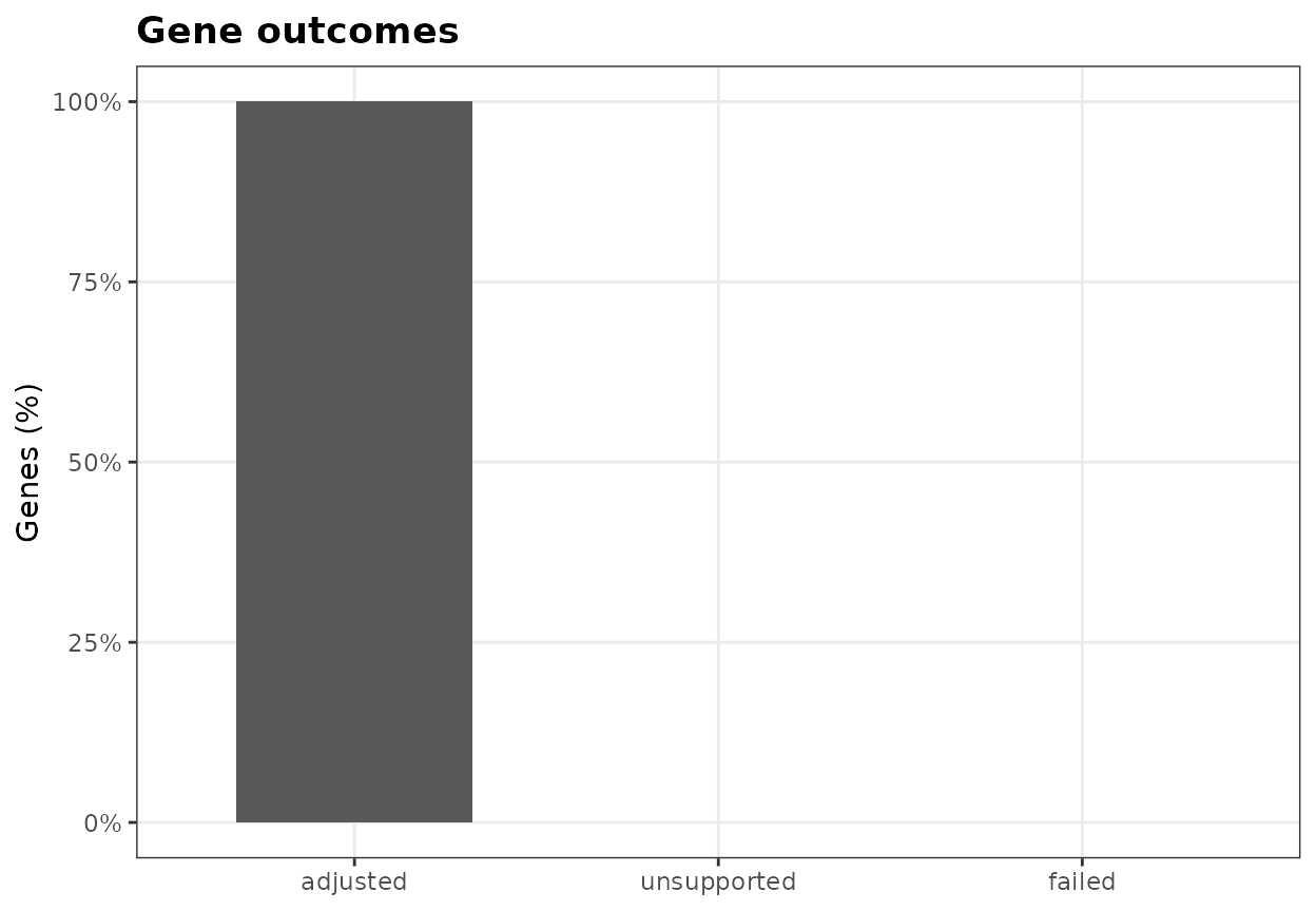

The outcome counts distinguish adjusted, unsupported, and failed genes. An unsupported gene lacks sufficient support for a reliable correction; it is not the same as a failed numerical correction. These categories correspond to the status recorded in fit@gene_status.

Customizing an individual plot

Individual diagnostics are ordinary ggplot objects, so standard ggplot2 layers, labels, scales, and themes can be added directly.

p <- ggplot2::autoplot(fit, type = "confidence")

p +
  ggplot2::labs(title = "Confidence by source batch") +
  ggplot2::theme(
    axis.text.x = ggplot2::element_text(angle = 45, hjust = 1)
  )

Which view should I use?

Use ggplot2::autoplot(fit) for routine post-fit QC and a specific type when inspecting or presenting one diagnostic. Use the underlying tables when numeric detail is required:

fit@diagnostics$batches
fit@diagnostics$correction_confidence
fit@diagnostics$batch_contrasts
fit@diagnostics$outcomes

These plots show reference-selection behavior, correction support, empirical-Bayes moderation, and adjustment outcomes. They do not independently demonstrate absence of residual confounding, complete removal of unwanted structure, or preservation of every biological signal. For differential- expression inference, use the original counts and model batch directly in the inferential design, as described in Getting started.